import matplotlib.pyplot as plt
plt.ion()
plt.subplot(1,1,1)
plt.plot([1,2,3])

#####################################################################
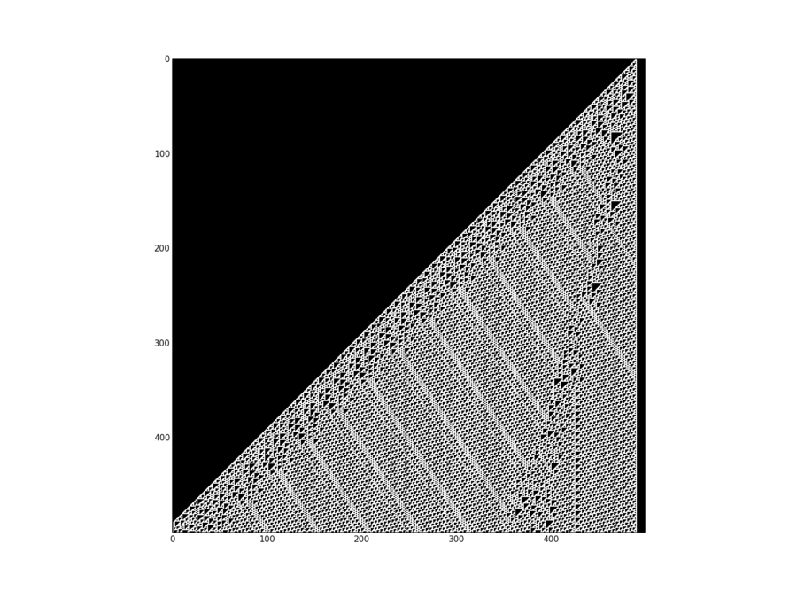
# Generate an image and pyplot.show it
#
# generate and plot a cellular automaton run
# (Rule 110: https://en.wikipedia.org/wiki/Rule_of_110)

##############################
# Import libraries

import matplotlib.pyplot as plt
import numpy as np

##############################
# Initialize image variable

# Dimension of the image
dim_row = 500; dim_col = 510

# An image is a numpy.array for matplotlib
img =  np.zeros((dim_row, dim_col))

##############################
# Run Rule 110

# Set first cell alive
img[0,dim_col-10] = 1

# Function computing next cell (Rule 110)
def next_cell(cs):
    c = cs[1] + cs[2]
    if 1 < c: c = 1 - cs[0]
    return c

# Let the cells evolve
for i in xrange(dim_row-1):
    for j in xrange(1,dim_col-1):
        img[i+1,j] = next_cell(img[i,j-1:j+2])

##############################
# Plotting

# Plot the cells    
imgplot = plt.imshow(img)
# We wont to see pixels
imgplot.set_interpolation('nearest')
# Rule 110 shuld be black and white
imgplot.set_cmap('bone')
# Let's see
plt.show()

##############################################################################
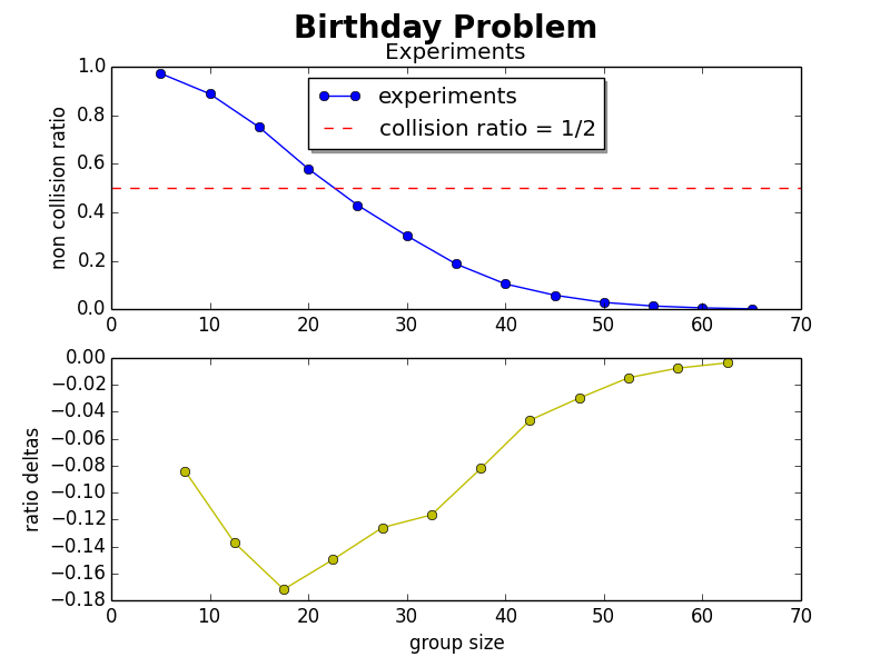
# Some plots of the birthday problem (see MAT101 Summary Week 3)
# Group size versus non collision ratio

##############################
# Import libraries
import matplotlib.pyplot as plt
from birthday import birthday_experiment

##############################
# Set up birthday experiments
number_groups = 10**4
size_min = 5; size_max = 65; delta = 5
group_sizes = range(size_min, size_max+delta, delta)

##############################
# Do the experiments
experiments = []
print 'Group sizes: ', group_sizes
for size in group_sizes:
    # Display some status
    print 'group size: ', size
    experiments.append(birthday_experiment(size, number_groups))

##############################
# Plots
fig = plt.figure(1)
fig.suptitle('Birthday Problem', fontsize=20, fontweight='bold')

# Two axes with common x-axis
# The first plot shows the experiment results
ax1 = fig.add_subplot(2,1,1)
ax1.plot(group_sizes, experiments, 'o-', label='experiments')

# A line showing the 1/2 collision ratio
ax1.axhline(.5, color= 'red', linestyle='--',\
            label='collision ratio = 1/2')

# Title and legend
ax1.set_title('Experiments')
ax1.set_ylabel('non collision ratio')
ax1.legend(loc='upper center', shadow=True)

# The second plot shows the deltas in the experiment results.
# The two plots share the x-axis: "sharex=ax1"
ax2 = fig.add_subplot(2,1,2, sharex=ax1)
ax2.plot([g+delta/2. for g in group_sizes[0:-1]],\
             [experiments[i]-experiments[i-1] \
                 for i in range(1,len(experiments))], 'y-o')

# Labels
ax2.set_xlabel('group size')
ax2.set_ylabel('ratio deltas')

# Let's see
plt.show()



##############################################################################
# This code wraps up the birthday experiment in a function
# Original code from the MAT101 Summary week 3

# Here is the dedication from the original file:

# Today is 25.09.2013, my birthday.
# This example file is dedicated to my friends Andreas and Catheline, and 
# their daughter who might or might not be born at this moment...
# She is very close, but she has only a few hours left if she wants to
# discover our world today, on the same date as me :-)
# Paul

import random

def birthday_experiment(group_size, number_groups):
    """
    Computes repeatedly the birthday experiment and returns the amount of runs
    without collision.
    group_size: group size used for each experiment
    number_groups: amount of experiments
    returns: #(experiments without collision)/#(experiments)
    """
    without_collision = 0
    for group_id in range(number_groups):          
        birthdays = []
        for person in range(group_size):
            birthday = random.randint(1, 365)
            if birthday in birthdays:
                break
            else:
                 birthdays.append(birthday)
        else:
            without_collision += 1
    return float(without_collision)/number_groups

##############################################################################
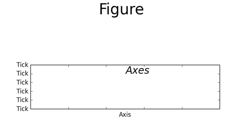
# Label the artist elements

import matplotlib.pyplot as plt

#############################
# Figure
# Instantiate
fig = plt.figure("Artist Elements")
# Add component name as subtitle
fig.suptitle('Figure', fontsize=30)

#############################
# Axes
# Instantiate
ax = fig.add_subplot(212)
# Add component name as text
ax.text(0.5, 0.8, 'Axes', fontsize=20, style='italic')

#############################
# Axis
# Get x/y-axis objects
xaxis = ax.xaxis
yaxis = ax.yaxis
# Get x-axis label
label = xaxis.get_label()
# Set x-axis label
label.set_text('Axis')

#############################
# Tick
# Import ticker module
import matplotlib.ticker as ticker
# Set y-axis tick labels
formatter = ticker.FormatStrFormatter('Tick')
yaxis.set_major_formatter(formatter)
# Disable xaxis tick labels
ticks = xaxis.get_major_ticks()
for t in ticks:
    t.label1On = False
    t.label2On = False

# Let's see
plt.show()

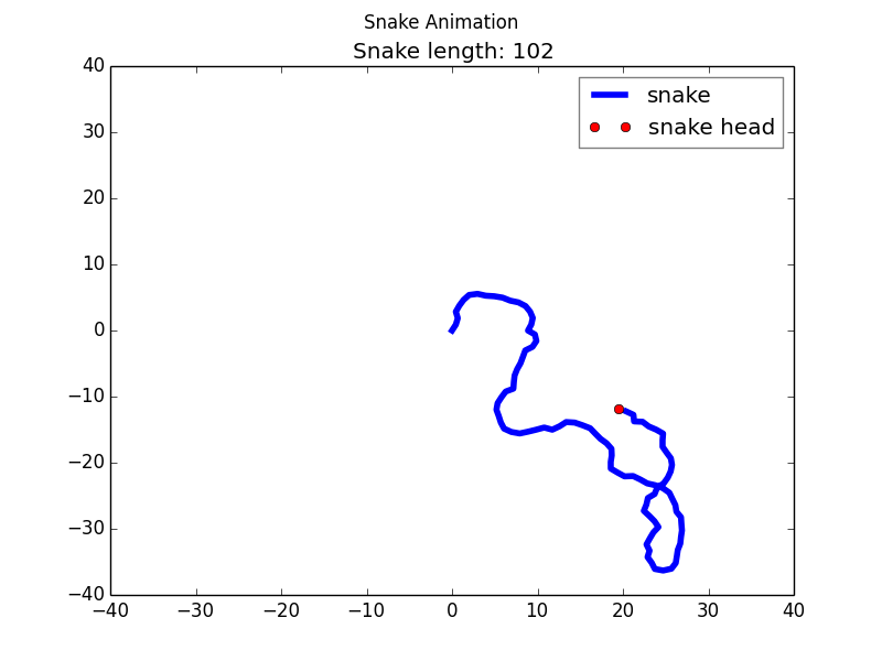
"""Snake animation as a matplotlib.animation example"""

import matplotlib.pyplot as plt
import matplotlib.animation as animation
import numpy as np
import random

#############################
# Helper functions

def limit_cage(position, cage_size):
    '''Limits position to be inside the cage'''
    return min(max(-cage_size+.5, position), cage_size-.5)

def snake_step(pos_x, pos_y, snake):
    '''Coumputes next head position'''
    snake['speed_angle'] += (random.gauss(0, .5))
    pos_x += np.sin(snake['speed_angle'])
    pos_y += np.cos(snake['speed_angle'])
    new_pos_x = limit_cage(pos_x, snake['cage_size'])
    new_pos_y = limit_cage(pos_y, snake['cage_size'])
    if pos_x != new_pos_x or pos_y != new_pos_y:
        snake['speed_angle'] += np.pi/2.
    return new_pos_x, new_pos_y

def update(num, snake):
    '''Computes next frame'''
    # Get snake head position
    snake_head_x = snake['head'].get_xdata()[0]
    snake_head_y = snake['head'].get_ydata()[0]

    # Add snake head point to snake body
    snake['body'].set_xdata(np.append(snake['body'].get_xdata(), snake_head_x))
    snake['body'].set_ydata(np.append(snake['body'].get_ydata(), snake_head_y))

    # Generate next snake head position
    snake_head_x, snake_head_y = snake_step(snake_head_x, snake_head_y, snake)
    snake['head'].set_xdata([snake_head_x])
    snake['head'].set_ydata([snake_head_y])

    # Update the title
    ax1.set_title("Snake length: "+str(num))

#############################
# Setup the figure
fig = plt.figure()
fig.suptitle("Snake Animation")

# Just one plotting area
ax1 = fig.add_subplot(1, 1, 1)

# The plot range
cage_size = 40
plt.xlim(-cage_size, cage_size)
plt.ylim(-cage_size, cage_size)

# Snake body
snake_body, = ax1.plot([], [], 'b', label='snake', linewidth=4)
# Snake head
snake_head, = ax1.plot([0.0], [0.0], 'ro', label='snake head')

# Legend
leg = ax1.legend()
leg.get_frame().set_alpha(0.5)

# The snake as dictionary
snake = {'head': snake_head, \
         'body': snake_body, \
         'speed_angle': 0, \
         'cage_size': cage_size}

# Generates the animation
ani = animation.FuncAnimation(fig, \
                              update, \
                              interval=50, \
                              fargs=[snake], \
                              blit=False, \
                              repeat=False)
#ani.save('mci_plot.avi', dpi=180) # matplotlib version 1.3.1
plt.show()

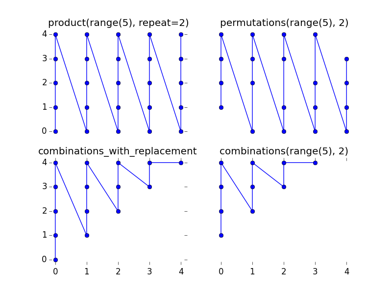
import itertools as it
import matplotlib.pyplot as plt

n = 5 
fig = plt.figure()
ax1 = fig.add_subplot(2,2,1, title="product(range("+str(n)+"), repeat=2)")
plt.plot(*it.izip(*it.product(range(n), repeat=2)), marker='o')
ax2 = fig.add_subplot(2,2,2, sharex=ax1, sharey=ax1, title="permutations(range("+str(n)+"), 2)")
plt.plot(*it.izip(*it.permutations(range(n), 2)), marker='o')
ax3 = fig.add_subplot(2,2,3, sharex=ax1, sharey=ax1, title="combinations_with_replacement")
plt.plot(*it.izip(*it.combinations_with_replacement(range(n), 2)), marker='o')
ax4 = fig.add_subplot(2,2,4, sharex=ax1, sharey=ax1, title="combinations(range("+str(n)+"), 2)")
plt.plot(*it.izip(*it.combinations(range(n), 2)), marker='o')
ax1.set_xlim(-.2, n-1+.2)
ax1.set_ylim(-.2, n-1+.2)

ax1.set_frame_on(False)
ax2.set_frame_on(False)
ax3.set_frame_on(False)
ax4.set_frame_on(False)
ax1.axes.get_xaxis().set_visible(False)
ax2.axes.get_xaxis().set_visible(False)
ax2.axes.get_yaxis().set_visible(False)
ax4.axes.get_yaxis().set_visible(False)

plt.show()